Build a CSV Sales Toolkit : Day 2 - Sales Analyzer & Report

Today we build a Python program that loads a messy CSV, see it in a table, click a button, and watch the data transform — bad values fixed, missing cells filled.

Projects in this week’s series:

This week, we build a CSV Sales Toolkit that cleans messy data, generates insightful reports, and processes whole folders of files at once — the exact workflow of real data work.

• Day 1: Visual CSV Cleaner

• Day 2: Sales Analyzer & Report (Today)

• Day 3: Batch CSV Processor

View All Projects This Week

Today’s Project

Yesterday we cleaned the data. Today we make it talk. Clean data is only useful if it tells you something — so today we build a Sales Analyzer that takes orders_clean.csv and computes the numbers a business actually cares about: total revenue, best-selling products, revenue by category, daily trends, and average order value.

The result is a formatted text report you can read at a glance or email to someone — turning a spreadsheet of rows into actual answers.

Project Task

Build a sales analyzer that:

• Loads the cleaned orders CSV from Day 1

• Separates completed orders from cancelled ones

• Calculates headline metrics: total revenue, order count, average order value

• Finds the best-selling products (by quantity and by revenue)

• Breaks revenue down by category

• Computes a daily sales trend

• Calculates the cancellation rate

• Formats everything into a clean, readable report

• Saves the report to a text file

This project gives you hands-on practice with pandas aggregation, groupby, sorting, filtering, and turning raw numbers into a formatted business report — the analysis half of real data work.

Expected Output

Running the analyzer:

python analyze_sales.py

Console Output (and saved report):

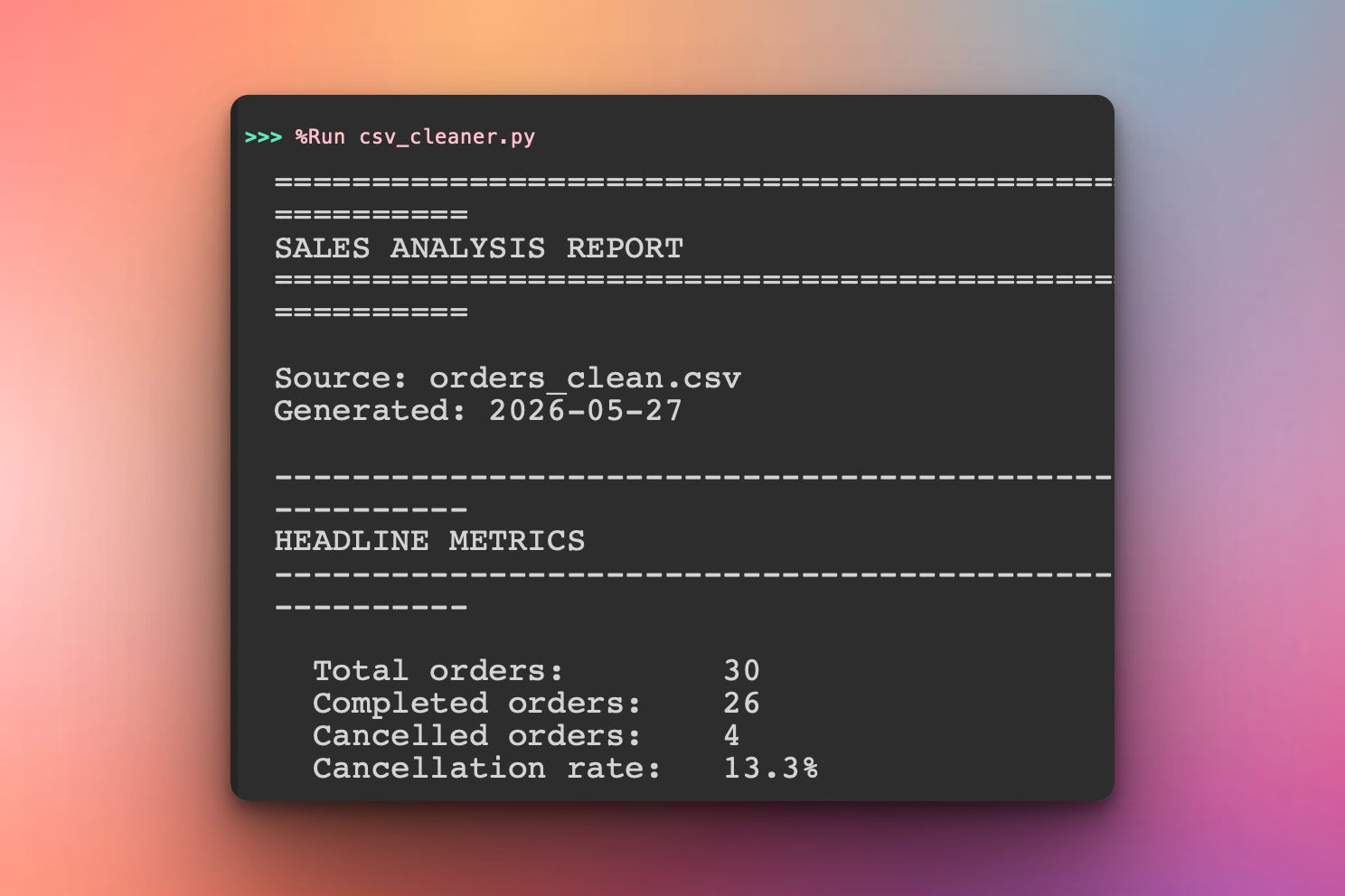
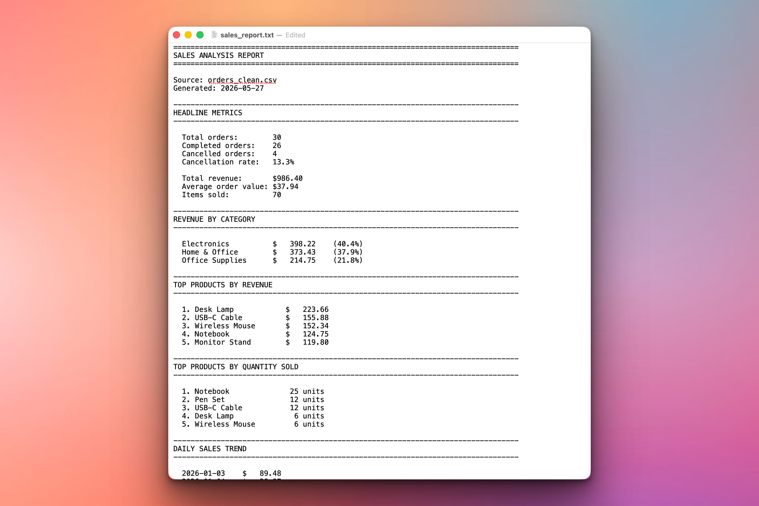
The same text is printed to the console and saved as sales_report.txt — readable, shareable, done.

Setup Instructions

Install pandas:

pip install pandas

Get the data file:

You need orders_clean.csv — the output of Day 1. Run the Day 1 cleaner first, or use the cleaned file provided below:

Place the orders_clean.csv file in the same folder as the script.

Run the Python script:

python analyze_sales.py

The script reads orders_clean.csv and writes sales_report.txt.

Understanding Why Clean Data Matters Here

Day 1 wasn’t busywork — today is where it pays off. Every calculation below depends on the cleaning:

• Total revenue sums total_price — only possible because prices are real numbers, not $12.99 text.

• Revenue by category groups by category — only gives 3 groups because we standardized the capitalization.

• Completed vs. cancelled filters on status — only works because we made the status values consistent.

Analysis on dirty data produces confidently wrong answers. That’s worse than no answer. Clean first, analyze second — always.

Understanding Loading and Filtering

We start by loading the clean CSV and splitting it by status. Most metrics should count completed orders only — a cancelled order earned no revenue:

import pandas as pd

df = pd.read_csv("orders_clean.csv")

# Split by status
completed = df[df["status"] == "completed"]
cancelled = df[df["status"] == "cancelled"]

df[df["status"] == "completed"] is boolean filtering — the inner part builds a column of True/False, and the outer part keeps only the True rows. This is the single most common pandas operation, and it’s how we make sure cancelled orders don’t inflate revenue.

Understanding Headline Metrics

The top-level numbers are simple aggregations on the completed orders:

total_revenue = completed["total_price"].sum()
order_count = len(completed)
items_sold = completed["quantity"].sum()

# Average order value — guard against dividing by zero
average_order = total_revenue / order_count if order_count else 0

# Cancellation rate as a percentage
cancellation_rate = len(cancelled) / len(df) * 100

Each metric is one line. .sum() adds a column, len() counts rows. The only subtlety is guarding the division — if order_count else 0 prevents a crash if there are no completed orders. Defensive arithmetic like this is what separates a script that works on your data from one that works on any data.

Understanding groupby for Category Revenue

To break revenue down by category, we use groupby — pandas’ tool for “split into groups, then calculate per group”:

category_revenue = (
    completed.groupby("category")["total_price"]
    .sum()
    .sort_values(ascending=False)
)

Read it as a pipeline:

1. groupby("category") — split the rows into one group per category.

2. ["total_price"] — we only care about the price column.

3. .sum() — total it within each group.

4. .sort_values(ascending=False) — order the result, biggest first.

The result is a Series: category names on the left, total revenue on the right. This four-step pattern — group, select, aggregate, sort — is the backbone of nearly every report you’ll ever write.

Understanding Top Products

“Best-selling” has two meanings, and a good report shows both. Some products sell in high volume; others bring in more money. Same groupby pattern, different column:

# By revenue — which products earn the most money
top_by_revenue = (
    completed.groupby("product")["total_price"]
    .sum()
    .sort_values(ascending=False)
    .head(5)
)

# By quantity — which products sell the most units
top_by_quantity = (
    completed.groupby("product")["quantity"]
    .sum()
    .sort_values(ascending=False)
    .head(5)
)

.head(5) keeps only the top five after sorting. Showing both lists is genuinely useful: a cheap product can top the quantity list while barely registering on revenue — that contrast is an insight, not just a number.

Understanding the Daily Trend

To see sales over time, we group by date. The order_date column is text, so we convert it to real dates first — that makes it sort chronologically and behave correctly:

completed = completed.copy()
completed["order_date"] = pd.to_datetime(completed["order_date"])

daily_sales = (
    completed.groupby("order_date")["total_price"]
    .sum()
    .sort_index()
)

# The single best day
best_day = daily_sales.idxmax()       # the date with the highest total
best_amount = daily_sales.max()        # that highest total

Two new tools here:

• pd.to_datetime turns date text into real date objects, so 2026-01-09 sorts after 2026-01-08, not alphabetically.

• .idxmax() returns the index label of the maximum value — here, the date of the best day — while .max() returns the value itself. The pair answers “what was the best day, and how good was it?”

Note the .copy() — when you take a filtered slice of a DataFrame and then modify it, pandas warns you. .copy() makes a clean, independent copy so the modification is unambiguous and warning-free.

Understanding Formatting the Report

Raw numbers aren’t a report — formatting makes them readable. Python’s f-strings give you fine control over alignment and number display:

# Currency: 2 decimals, comma thousands separator
print(f"  Total revenue:  ${total_revenue:,.2f}")
# -> "  Total revenue:  $986.40"

# Percentage: 1 decimal place
print(f"  Cancellation rate:  {cancellation_rate:.1f}%")
# -> "  Cancellation rate:  20.0%"

# Aligned columns: pad the name to a fixed width
for product, revenue in top_by_revenue.items():
    print(f"  {product:<20} ${revenue:>9,.2f}")

The format codes earn their keep:

• :,.2f — comma thousands separator, exactly 2 decimals (money).

• :.1f — 1 decimal place (percentages).

• :<20 — left-align in a 20-character space (product names line up).

• :>9 — right-align in a 9-character space (numbers line up by the decimal).

Aligned columns are the difference between a report that looks professional and one that looks like a data dump.

Understanding Building Report Sections

Rather than print scattered everywhere, we build the report as a list of text lines, then join it once at the end. This way the same text goes to both the console and the file:

def build_report(df):
    lines = []
    lines.append("=" * 80)
    lines.append("SALES ANALYSIS REPORT")
    lines.append("=" * 80)
    lines.append("")
    # ... append every section ...
    return "\n".join(lines)

Collecting lines in a list and "\n".join()-ing them at the end is cleaner than dozens of print calls. You build the report once, as a string — then you can print it, save it, or both, with no duplication.

Understanding Saving the Report

Writing the finished report to a text file is a few lines with a with block:

report_text = build_report(df)

print(report_text)                       # show it on screen

with open("sales_report.txt", "w") as f: # and save it to a file
    f.write(report_text)

The with open(...) block handles the file safely — it’s automatically closed even if something goes wrong. Because build_report returned one string, sending it to both the screen and the file is trivial. A .txt report is something a non-technical person can open, read, and forward — which is often the whole point of doing the analysis.

Practical Use Cases

1. Weekly or monthly sales summaries:

Run the analyzer on the latest data, get a report ready to send to your team.

2. Spotting your best products:

The revenue vs. quantity lists reveal which products to promote or restock.

3. Tracking cancellation problems:

A rising cancellation rate is an early warning worth watching.

4. Finding peak sales days:

The daily trend shows when customers buy — useful for planning promotions.

5. Foundation for Day 3:

Tomorrow we run this analysis across a whole folder of monthly files at once.

Coming Tomorrow

Tomorrow is the finale: the Batch CSV Processor. Instead of one file, you’ll point the tool at a folder of monthly sales CSVs — it cleans every one, analyzes them all, merges the data, and produces a single consolidated multi-month report. Real batch processing.

View Code Evolution

Compare today’s analyzer with yesterday’s cleaner and see how clean, typed data turns directly into meaningful business metrics.