Build a CSV Sales Toolkit : Day 3 - Batch CSV Processor

Today’s tool points at a folder of monthly sales CSVs, cleans every one, combines them all into a single dataset, and produces a consolidated multi-month report.

Projects in this week’s series:

This week, we build a CSV Sales Toolkit that cleans messy data, generates insightful reports, and processes whole folders of files at once — the exact workflow of real data work.

• Day 1: Visual CSV Cleaner

• Day 2: Sales Analyzer & Report

• Day 3: Batch CSV Processor (Today)

View All Projects This Week

Today’s Project

Welcome to the finale. You have a cleaner and an analyzer. Today they grow up. Instead of working on one file at a time, today’s tool points at a folder of monthly sales CSVs, cleans every one, combines them all into a single dataset, and produces a consolidated multi-month report — with per-month comparisons, growth percentages, and a full-period summary.

This is the moment your script becomes a tool someone could automate. Drop a new month’s file into the folder, run the script, get the updated report. That’s how real data work scales.

Project Task

Build a batch CSV processor that:

• Discovers every CSV in a designated folder automatically

• Cleans each file using the Day 1 cleaning pipeline

• Reports the result of each file (rows, missing values fixed)

• Continues to the next file if one fails, instead of crashing

• Merges all cleaned data into a single combined DataFrame

• Runs the Day 2 analysis on the combined data

• Adds per-month aggregates (revenue per month, month-over-month change)

• Identifies the best month, top product overall, and trends

• Saves both the combined CSV and the consolidated report

• Prints a progress summary as it works

This project gives you hands-on practice with pathlib for folder scanning, batch file handling, robust error handling, pd.concat for combining DataFrames, time-grouped aggregations with dt.to_period, and turning your earlier scripts into reusable functions.

Expected Output

Folder structure before running:

monthly_sales/
├── sales_2026_01.csv     (30 orders, messy)
├── sales_2026_02.csv     (25 orders, messy)
├── sales_2026_03.csv     (27 orders, messy)
└── sales_2026_04.csv     (28 orders, messy)

Running the processor:

python batch_process.py

Console Output:

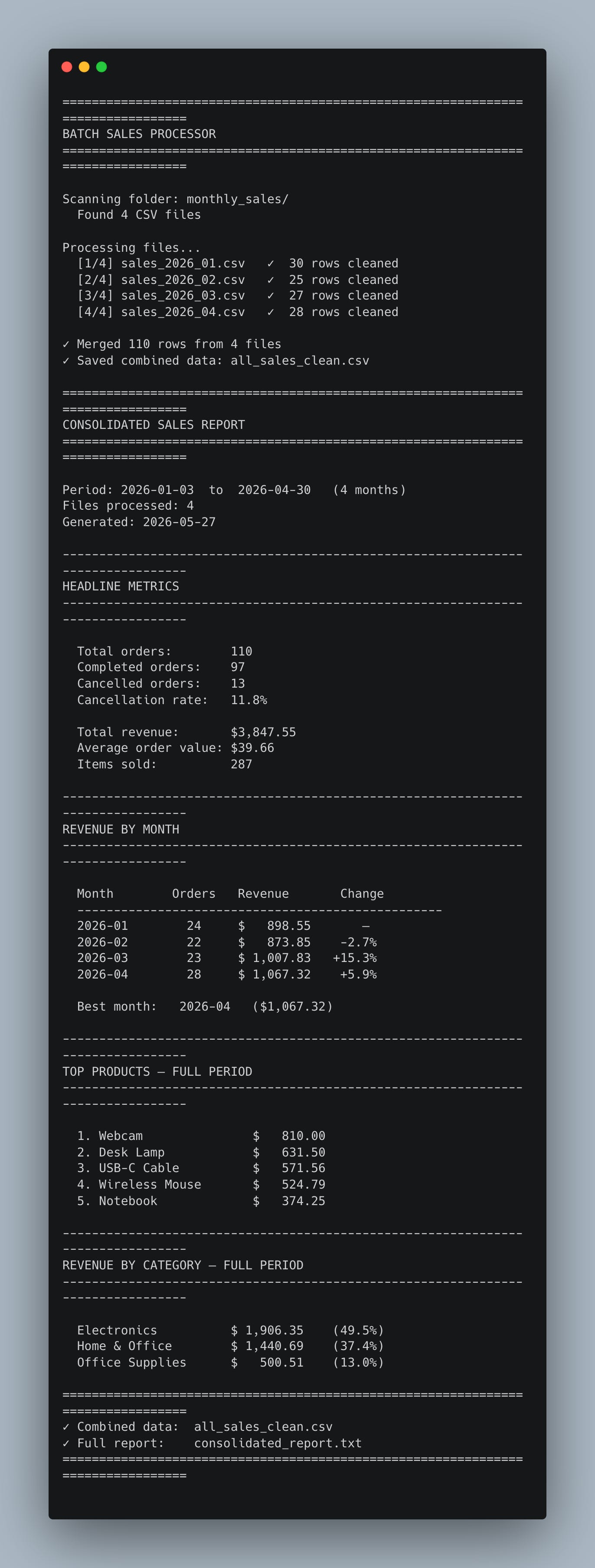
You drop a fifth month into the folder next quarter — and rerunning produces an updated five-month report with no changes to the code. That’s the win.

Setup Instructions

Install pandas:

pip install pandas

Get the data files:

Download the monthly_sales/ folder:

It contains four monthly CSVs. Place the folder next to your script.

Run it:

python batch_process.py

The script reads every CSV in monthly_sales/ and writes two new files: all_sales_clean.csv (the merged clean data) and consolidated_report.txt (the report).

Understanding Folder Scanning with pathlib

The first batch trick is finding the files automatically. We don’t hardcode filenames — we ask the folder what’s in it. pathlib makes this elegant:

from pathlib import Path

folder = Path("monthly_sales")
csv_files = sorted(folder.glob("*.csv"))

print(f"Found {len(csv_files)} CSV files")
for path in csv_files:
    print(f"  {path.name}")

Three things to know:

• Path("monthly_sales") — pathlib’s modern, OS-aware way to point at a folder.

• .glob("*.csv") — returns every file matching the pattern.

• sorted(...) — files come back in filesystem order, which can vary. Sorting alphabetically gives you predictable chronological order when filenames include dates.

Adding a new monthly file later is now a non-event. The script discovers it automatically.

Understanding Reusable Cleaning Functions

We need the Day 1 cleaning logic — but as a function, not a GUI button. So we lift it into a standalone helper:

TEXT_COLUMNS = ["customer_name", "product", "category", "status"]

def clean_dataframe(df):
    """Apply every cleaning step from Day 1 and return the result."""
    for col in TEXT_COLUMNS:
        df[col] = df[col].astype(str).str.strip()

    df["category"] = df["category"].str.title()
    df["status"] = df["status"].str.lower()

    df["unit_price"] = (
        df["unit_price"].astype(str)
        .str.replace("$", "", regex=False)
        .str.replace(",", "", regex=False)
    )
    df["unit_price"] = pd.to_numeric(df["unit_price"], errors="coerce")

    df["quantity"] = pd.to_numeric(df["quantity"], errors="coerce")
    df["quantity"] = df["quantity"].fillna(1).astype(int)

    category_avg = df.groupby("category")["unit_price"].transform("mean")
    df["unit_price"] = df["unit_price"].fillna(category_avg).round(2)

    df["total_price"] = (df["quantity"] * df["unit_price"]).round(2)

    return df

This is the same logic as Day 1, packaged so it can be called over and over. That’s the broader lesson: a function you wrote for one file works for a thousand, the moment you stop hardcoding the data and start passing it as an argument.

Understanding the Batch Loop

The heart of batch processing is the loop. For each file: load, clean, collect. The key habit is defensive error handling — one bad file should not destroy the entire run:

cleaned_dfs = []
failures = []

for i, path in enumerate(csv_files, 1):
    try:
        df = pd.read_csv(path)
        df = clean_dataframe(df)
        cleaned_dfs.append(df)
        print(f"  [{i}/{len(csv_files)}] {path.name}   ✓  {len(df)} rows cleaned")
    except Exception as e:
        failures.append((path.name, str(e)))
        print(f"  [{i}/{len(csv_files)}] {path.name}   ✗  {e}")

Two important moves:

• try/except around each file — if one CSV is corrupt or has unexpected columns, the loop logs the failure and continues. The other files still process.

• failures list — collecting errors instead of letting them kill the script means you get a complete picture of what happened, even when some files broke.

A batch tool that crashes on the third file out of fifty is barely better than running them manually. Robustness is the feature.

Understanding pd.concat for Merging

After cleaning, we combine the per-file DataFrames into one. pd.concat is the tool:

combined = pd.concat(cleaned_dfs, ignore_index=True)
combined.to_csv("all_sales_clean.csv", index=False)

pd.concat stacks DataFrames vertically — row after row — as long as they share columns. ignore_index=True is important: without it, you keep each file’s original row indexes (0, 1, 2... then 0, 1, 2... again). With it, you get a single fresh sequence — much easier to work with.

The merged file is also a deliverable. Now you have a single clean CSV holding every month’s data, ready for any future analysis.

Understanding Period Grouping

The headline new capability today is monthly comparisons. With the merged data, we can group by month using pandas’ time-period feature:

combined["order_date"] = pd.to_datetime(combined["order_date"])

monthly = (
    completed.assign(month=completed["order_date"].dt.to_period("M"))
    .groupby("month")
    .agg(
        orders=("order_id", "count"),
        revenue=("total_price", "sum"),
    )
)

Two new ideas here:

• .dt.to_period("M") — converts a date like 2026-01-15 into the period 2026-01. Every date in January becomes the same period, which is exactly what you need to group by month.

• .agg(name=(column, function), ...) — the named-aggregation form of agg. You get to name each output column and pick what it’s computed from, in one clean call. Much more readable than the older positional form.

The result is a small DataFrame with one row per month, ready to compare.

Understanding Month-over-Month Change

A monthly total tells you what happened. A month-over-month change tells you the direction. Pandas’ pct_change() makes this a one-liner:

monthly["change"] = monthly["revenue"].pct_change() * 100
# Output:
# 2026-01     —      (first month, no prior to compare to)
# 2026-02   -2.7%
# 2026-03  +15.3%
# 2026-04   +5.9%

pct_change() returns the percentage change between each row and the one before it. The first row gets NaN — there’s no earlier value to compare to — which we display as an em-dash.

This single column turns a list of monthly revenues into a story: “Dipped in Feb, surged 15% in March, and kept climbing.” That’s the kind of sentence reports are supposed to enable.

Understanding Formatting the Monthly Table

The monthly section needs careful column alignment to look like a real report:

lines.append("  Month        Orders   Revenue       Change")
lines.append("  " + "-" * 48)

for month, row in monthly.iterrows():
    change = row["change"]
    if pd.isna(change):
        change_str = "    —"            # first month, nothing to compare to
    else:
        sign = "+" if change >= 0 else ""
        change_str = f"{sign}{change:.1f}%"

    lines.append(
        f"  {str(month):<10}"
        f"  {int(row['orders']):>4}"
        f"     ${row['revenue']:>8,.2f}"
        f"   {change_str:>6}"
    )

A few details earn their place:

• pd.isna(change) — the safe way to check for missing values. (change == NaN always returns False — never use == for NaN.)

• "+" if change >= 0 else "" — manually prepending + makes positive numbers visually distinct from negative ones at a glance.

• {...:<10} / {...:>4} / {...:>8,.2f} — left- and right-alignment with widths. The column headers and the data rows use the same widths, so everything lines up.

These small touches turn raw numbers into a table that reads like something from a real product.

Understanding Why This Architecture Works

Look at the three days side by side:

• Day 1 built a clean_dataframe workflow inside a GUI.

• Day 2 built build_report from clean data.

• Day 3 wraps both in a loop over a folder.

Each layer was rewritten exactly once: when its job changed. The cleaning logic didn’t change today — we just call it in a loop. The reporting structure didn’t change much either — we added monthly comparisons. Most of today’s code is glue: scanning a folder, iterating, concatenating, formatting. That’s a real pattern for building software: solve one case well, then loop the solution.

Practical Use Cases

1. Monthly business reporting:

Drop each new month's export into the folder, rerun, get an updated report — forever.

2. Year-end consolidation:

Process 12 monthly files into one yearly summary, with month-over-month growth.

3. Multi-source data merging:

Combine exports from different stores, regions, or systems into one analysis.

4. Building data pipelines:

The pattern (discover → clean → merge → analyze) is the skeleton of every ETL job.

5. Automated jobs:

Schedule this script and it generates fresh reports nightly without supervision.

What You’ve Accomplished This Week

🎉 Congratulations! You’ve built a complete CSV Sales Toolkit.

• Day 1: Visual CSV cleaner — fixes real-world data mess with a click

• Day 2: Sales analyzer — turns clean data into business insights

• Day 3: Batch processor — scales the whole pipeline to a folder of files

You now have:

✅ Data cleaning skills — whitespace, casing, types, missing values, the real toolkit ✅ Aggregation skills — groupby, agg, pct_change, period grouping ✅ Batch processing skills — pathlib, looped error handling, pd.concat ✅ Report formatting skills — alignment, currency, percent, multi-section output ✅ A clean architecture — three layers, reused not rewritten

Real-world applications:

• 📊 Sales and finance reporting — exactly the workflow this teaches

• 🧾 Receipt or invoice consolidation — batch-clean and merge

• 🏷️ Inventory analysis — same patterns apply to product/stock data

• 📈 Marketing reporting — clean campaign exports, aggregate, compare

• 🤖 Personal automation — turn a 30-minute manual job into a 10-second script

Next steps:

• Add charts: matplotlib bar/line plots embedded in a PDF report

• Make it incremental: detect new files and only process those

• Schedule it: run nightly with cron, send the report by email

• Add forecasting: use the monthly trend to predict next month

• Database storage: write the cleaned merged data into SQLite for queries

You’ve built the foundation for a real data automation pipeline.

View Code Evolution

Compare today’s batch processor with the Day 1 cleaner and Day 2 analyzer — and see how a folder loop, robust error handling, and one good architecture turn a small script into a tool that scales.