

Visualizing the 2026 Eclipse with Python: Day 1 - Command-line eclipse info tool
Eight days from now mainland Europe gets its first total solar eclipse since 1999. Here’s the Python astronomy that tells you exactly what your city will see.

On August 12, the Moon’s shadow will sweep across Greenland, Iceland, and northern Spain — the first time mainland Europe has seen a total solar eclipse since 1999. Whether you’re in the path of totality, catching a 94% partial from Lisbon, or getting a thin 9% sliver in New York, exactly what you see depends on precise Sun-Moon geometry from your specific spot on Earth. And that geometry is computable — in Python — with the same JPL ephemeris data NASA uses.
This week we build a real astronomy tool. Day 1 is a Python CLI script that answers “what will I see from my location?” for any place on Earth — eclipse start, maximum, end, percentage of Sun covered, whether you’re in the path of totality. Day 2 wraps the astronomy in an interactive Streamlit web map: click anywhere on the world, get instant local eclipse timing. The astronomy is the hard part, and we do it once — Day 2 imports the same functions we build today.
Projects in this week’s series:
👉 Day 1: Command-line eclipse info tool (Today)
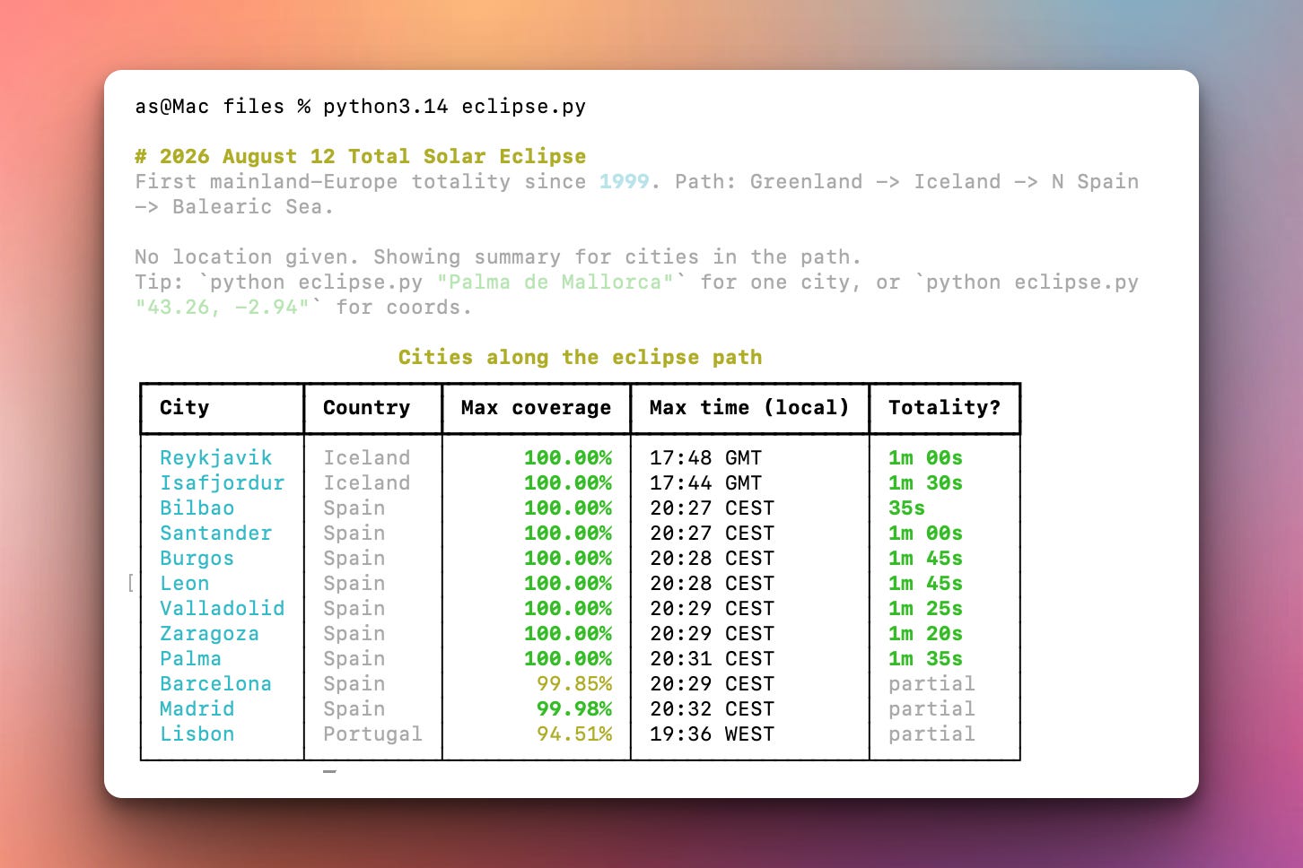
When the user runs the script with no arguments, it prints a colored summary table of all the major cities in the eclipse path — Reykjavik, Bilbao, Burgos, Zaragoza, Palma, plus nearby cities like Barcelona, Madrid, and Lisbon that get deep partials:
When they run it with a city name, for example:
python eclipse.py Madridor coordinates:
python eclipse.py "43.26, -2.94" they get a detailed report — start/max/end times in local timezone plus UTC, coverage percentage, magnitude, and totality duration if applicable:
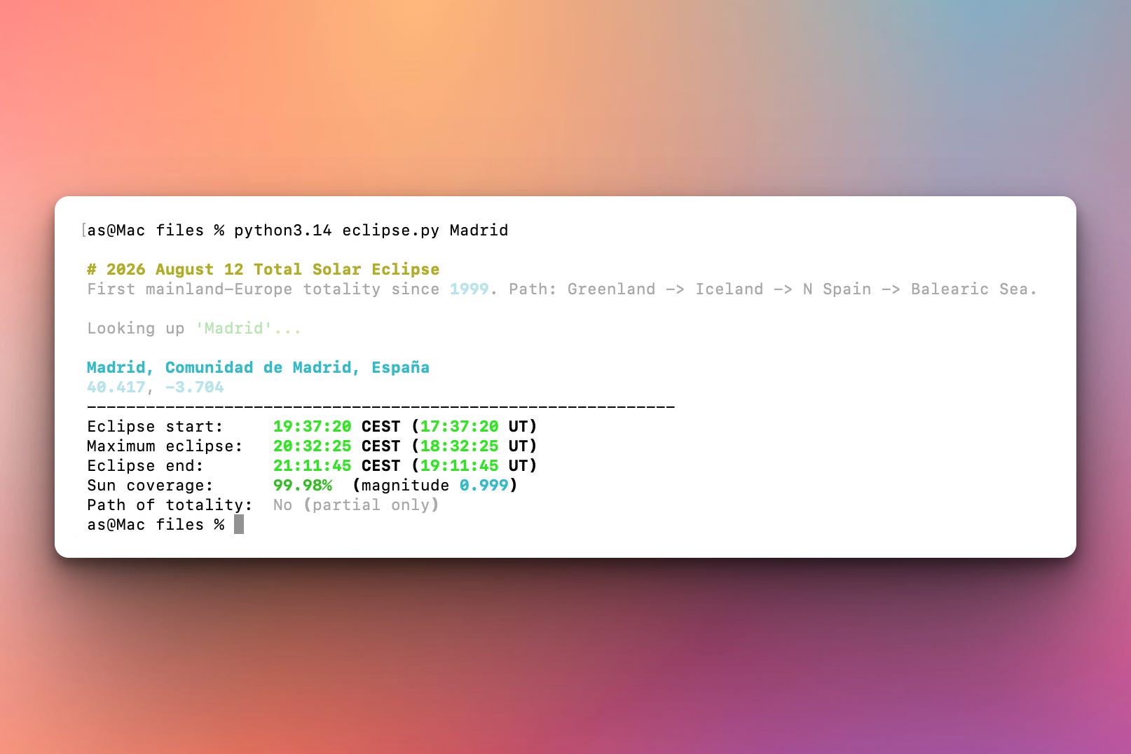
Everything is computed live from JPL ephemerides. Accurate to within seconds of NASA’s published numbers.
Day 2 (Tomorrow): Interactive Streamlit web map of the eclipse
Tomorrow we will use the astronomy engine, but wrapped in Streamlit + Folium. Full eclipse path drawn on an interactive world map — centerline and totality band. Click anywhere on Earth and the sidebar populates with local eclipse info computed live for that exact point. City search box (type “Rome” or “Boston” instead of clicking). Real-time countdown to the eclipse. Major cities pre-marked with popups:
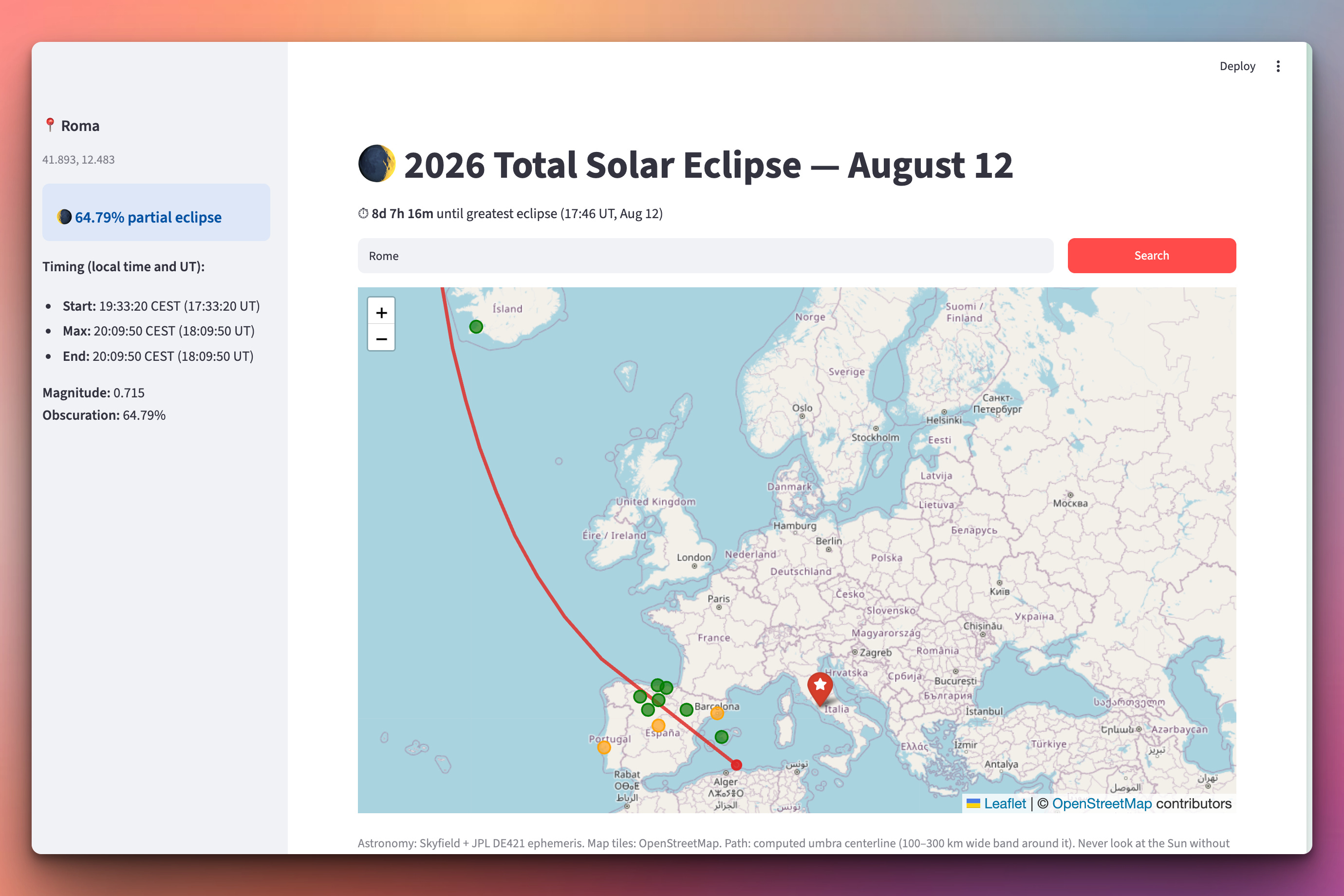
The map is the payoff of the week — turning terminal output into something you can share with your family, your students, or a WhatsApp group.
About the stack
Today’s script uses five packages, each doing one specific thing:
Skyfield is Python’s modern astronomy library. It reads JPL planetary ephemeris files — the same tables NASA uses to navigate spacecraft — and gives you sub-second-accurate positions of the Sun, Moon, planets, and satellites from any point on Earth at any time. This is real, professional-grade astronomy code. When you run it and get an eclipse timing, that timing is correct to within a second or two.
skyfield-data is a companion package that bundles the DE421 ephemeris file (about 17 MB of JPL data covering 1900–2050) as a Python package. Normally Skyfield downloads the file from JPL on first run; using skyfield-data means it just works offline, no download step, no waiting.
Rich is the library for beautiful terminal output in Python. Colored text, formatted tables, spinners, progress bars — one import and your CLI script suddenly looks professional instead of like a homework submission. The tables it produces are Unicode box-drawing characters that render perfectly in any modern terminal.
geopy does geocoding — city name to lat/lon. It’s a thin wrapper around Nominatim (OpenStreetMap’s free geocoder), so geopy.geocode("Bilbao") returns (43.263, -2.935) and works for any place OpenStreetMap knows about.
timezonefinder does the opposite of geocoding for time — given a lat/lon, it tells you the timezone. Purely offline, backed by polygon data for every timezone on Earth. We use this to convert Skyfield’s UTC timestamps into local time at the user’s chosen location, so “eclipse maximum at 18:27:20 UT” becomes “20:27:20 CEST” for a Spanish city and “17:48:00 GMT” for Reykjavik automatically.
The single-file philosophy stays
Everything — imports, constants, city list, astronomy math, geometry, formatting, CLI parsing — lives in one eclipse.py file. Around 400 lines total, organized in clearly-labeled sections. No config file, no separate modules, no folder hopping.
Setup Instructions
Install dependencies:
pip install skyfield skyfield-data rich geopy timezonefinder numpy
Six packages. The one to know about is skyfield-data — without it, Skyfield will download the JPL ephemeris file on first run (~17 MB, one-time). With it, the file lives inside the pip package and everything works offline.
Run it in one of the following ways:
python eclipse.py                       # summary table for cities in the path
python eclipse.py Bilbao                # detailed report for one city
python eclipse.py "Palma de Mallorca"   # quote names with spaces
python eclipse.py "43.26, -2.94"        # or pass raw coordinates
First run takes a couple of seconds to load the ephemeris and Rich; subsequent runs are near-instant.
Understanding the Astronomy
The whole eclipse question — from your specific location on Earth — reduces to one geometric question repeated over time: how much do the Sun’s and Moon’s apparent disks overlap as seen from your standing point?
Each disk has an angular size in the sky. The Sun’s angular radius from Earth is about 15.8 arcminutes (roughly a quarter of a degree). The Moon’s is almost identical — around 15.5 to 16.7 arcminutes depending on where the Moon is in its elliptical orbit. That near-perfect size match is why total solar eclipses exist at all: if the Moon were noticeably smaller in the sky, we’d only ever get annular eclipses; if noticeably larger, no “diamond ring” moment. It’s a coincidence of two body sizes and orbital distances that will end in about 600 million years as the Moon slowly drifts away.
For an eclipse from your location, the question is what fraction of the Sun’s disk area is covered by the Moon’s disk at each moment. When that fraction is 0, no eclipse. When it’s 1 and the disks are perfectly overlapping, totality. Everything between is a partial. Simple in principle. In practice, we need to know the exact angular positions of Sun and Moon as seen from your specific lat/lon at every moment during the event.
That’s what Skyfield gives us.
Understanding Skyfield
Skyfield is the professional-grade astronomy library for Python. Under the hood, it reads JPL DE421 — a giant table of planetary positions computed by NASA’s Jet Propulsion Laboratory for the years 1900 to 2050, accurate to sub-arcsecond. Every time we ask “where is the Moon right now?”, Skyfield interpolates through this table.
Three fundamental objects:
from skyfield.api import load, load_file, wgs84
from skyfield_data import get_skyfield_data_path
import os

# The ephemeris (planetary positions table).
bsp = os.path.join(get_skyfield_data_path(), 'de421.bsp')
ts = load.timescale()          # for building Time objects
eph = load_file(bsp)           # the JPL ephemeris

sun = eph['sun']
moon = eph['moon']
earth = eph['earth']
Then we build an observer — a point on Earth’s surface with a lat/lon:
observer = earth + wgs84.latlon(43.263, -2.935) # Bilbao
Now we can ask “what does the observer see?” at any time:
t = ts.utc(2026, 8, 12, 18, 27)              # Aug 12, 2026, 18:27 UT
sun_app = observer.at(t).observe(sun).apparent()
moon_app = observer.at(t).observe(moon).apparent()
The .apparent() at the end applies all the corrections that make astronomy hard: light-travel time (the Sun’s photons left it 8 minutes ago, the Moon’s about 1.3 seconds ago), aberration of light due to Earth’s motion, and the deflection of light passing near the Sun. Real, textbook astronomy.
From these, we can extract everything we need:
separation = sun_app.separation_from(moon_app)       # angular gap
sun_dist_km = sun_app.distance().km                  # for angular radius
sun_alt_deg = sun_app.altaz()[0].degrees             # is Sun above horizon?
Understanding Angular Radii
Physical radii are known constants — the Sun is about 695,700 km in radius, the Moon 1,737.4 km. Angular radius depends on how far away the object is at that moment. The formula:
sun_rad = np.arcsin(R_SUN_KM / sun_dist_km)     # radians
moon_rad = np.arcsin(R_MOON_KM / moon_dist_km)  # radians
Simple trigonometry. The Sun’s distance varies by about 3% over the year (Earth’s slightly elliptical orbit). The Moon’s distance varies by about 12% each month (much more elliptical orbit). These small variations are exactly what determines whether a given eclipse is total or annular — and what fraction of the Sun’s disk gets covered at maximum in a given place.
Understanding Vectorized Time
Naive approach: loop through 5040 times (7 hours × 720 samples/hour at 5s resolution), computing Sun and Moon positions at each. That’s slow.
Better approach: pass all 5040 times to Skyfield at once, as a numpy array:
minutes = np.arange(0, 7*60, 5/60)   # every 5 seconds for 7 hours
times = ts.utc(2026, 8, 12, 14, minutes)   # ONE Time object containing 5040 timestamps

sun_app = observer.at(times).observe(sun).apparent()      # 5040-point result
moon_app = observer.at(times).observe(moon).apparent()    # 5040-point result

seps = sun_app.separation_from(moon_app).radians          # numpy array
sun_dist_km = sun_app.distance().km                       # numpy array
Skyfield handles vectorized time natively — internally, everything is numpy arrays. Total runtime for computing the eclipse at one city: about 0.4 seconds. For all 12 cities in the table: about 5 seconds. Fast enough that you can compute it live in a web app (which is what we’ll do on Day 2).
Understanding Circle-Circle Intersection
Once we have angular separation d and angular radii R and r, we need the intersection area of two circles. This is a classic geometry problem with a well-known closed-form solution:
def circle_intersection_area(d, R, r):
    """Works elementwise on numpy arrays. Three cases:"""

    # Case 1: no overlap
    if d >= R + r: return 0

    # Case 2: one disk fully contains the other
    if d <= abs(R - r): return np.pi * min(R, r)**2

    # Case 3: partial overlap - standard formula
    part1 = r**2 * np.arccos((d**2 + r**2 - R**2) / (2*d*r))
    part2 = R**2 * np.arccos((d**2 + R**2 - r**2) / (2*d*R))
    part3 = 0.5 * np.sqrt((-d+r+R) * (d+r-R) * (d-r+R) * (d+r+R))
    return part1 + part2 - part3
The math looks intimidating but the shape is intuitive. part1 is the area of the moon’s disk chord cut by the sun’s disk. part2 is the same for the sun cut by the moon. part3 corrects for the overlap of those two chords (which would otherwise be double-counted). The intersection area is part1 + part2 - part3. It’s the same formula every graphics engine uses for lens-flare rendering and collision detection.
Divide the intersection area by the sun’s area, and you have obscuration — the fraction of the Sun’s disk covered by the Moon at any given moment. Multiply by 100, you have the percentage.
Understanding the Horizon Check
Geometry can happily tell you the Sun and Moon are perfectly aligned at 3 AM local time — but no eclipse is visible then because the Sun is on the other side of the Earth. Every eclipse calculation has to check whether the Sun is actually above the horizon:
sun_alt_deg = sun_app.altaz()[0].degrees   # array of altitudes
above_horizon = sun_alt_deg > 0
obscuration = np.where(above_horizon, obscuration, 0.0)
altaz() returns (altitude, azimuth, distance) — altitude is how high above the horizon, azimuth is compass direction. Above 0 means visible, below 0 means the Sun has set (or hasn’t risen yet). Any moment when the Sun is below the horizon has effective obscuration of zero — the eclipse might be “happening” geometrically, but it’s happening on the far side of the world.
This is exactly why the eclipse table shows different results for Sydney (Sun already set, no eclipse visible) versus NYC (Sun at 62° altitude, small partial eclipse visible) versus Bilbao (Sun at 8° altitude — near sunset but still up, gets full totality).
Understanding Timezone Conversion
Skyfield returns everything in UTC. But nobody thinks in UTC. When we report to the user, we want their local time. Two libraries:
timezonefinder takes a lat/lon and returns a timezone name:
from timezonefinder import TimezoneFinder
tf = TimezoneFinder()
tf.timezone_at(lat=43.263, lng=-2.935)   # 'Europe/Madrid'
tf.timezone_at(lat=64.147, lng=-21.940)  # 'Atlantic/Reykjavik'
It works entirely offline using polygon data of every timezone on Earth. Fast and reliable.
zoneinfo (Python stdlib since 3.9) converts UTC datetimes into that timezone:
from zoneinfo import ZoneInfo
local = utc_dt.astimezone(ZoneInfo('Europe/Madrid'))
Together, they let us take any (lat, lon, utc_datetime) triple and produce a properly-localized display like 20:27:20 CEST. Handles daylight saving automatically because that’s built into the timezone data.
Understanding Path of Totality
The path of totality is where the Moon’s disk completely covers the Sun’s disk. Geometrically: separation + sun_radius <= moon_radius. That is, even at the farthest edge of the Sun from the Moon’s center, the Sun’s edge is still inside the Moon’s disk.
total_mask = (seps + sun_rad <= moon_rad) & above_horizon
in_totality = bool(total_mask.any())

if in_totality:
    first_total = np.argmax(total_mask)
    last_total = len(total_mask) - 1 - np.argmax(total_mask[::-1])
    totality_seconds = (last_total - first_total) * SAMPLE_STEP_SECONDS
For Burgos, our tool reports 1m 45s of totality. NASA’s official prediction is 1m 42s. That 3-second discrepancy is our sampling resolution (5 seconds), not an astronomy error — the underlying JPL data is accurate to milliseconds. If you needed sub-second precision, you’d interpolate between grid points; for a human-readable report, 3 seconds is fine.
Practical Use Cases
Trip planning right now. If you’re anywhere in Europe on August 12 and want to know exactly what you’ll see from your Airbnb, run this script with your coordinates. Get the exact times, plan your dinner around them.
Teaching astronomy. This is one of the most compact “real astronomy” projects you can build in Python. Under 400 lines and it produces genuinely correct results. Assignable to students at any level: middle-schoolers can play with cities, undergrads can dig into the geometry, grad students can extend it to future eclipses (there’s a total in North America in August 2044).
Foundation for Day 2. Every function we built today gets reused tomorrow in the web map. compute_eclipse(lat, lon) becomes the callback when someone clicks the map. That’s the pedagogical arc of the week: build the engine on Day 1, wrap it in something beautiful on Day 2.
Coming Wednesday
Tomorrow we take today’s astronomy engine and wrap it in an interactive Streamlit web app with a Folium/Leaflet map. Full eclipse path drawn as centerline and totality band. Click anywhere on the world and the sidebar populates with local eclipse info computed live. City search box, countdown timer, popups on major cities. The full “wow” of the week.
If you want the map, upgrade here before Wednesday.
Solution
Below you will find the source code of this project which will produce the same output as shown in the screenshots in this post.
Get the source code here:
I love astronomy. Probably won't be able to see it in AZ. I guess I need to check out the program....