Web Scraping with BeautifulSoup: Day 3 - Search & Analyze the Scraped Data

Today we turn the CSV into an interactive command-line search engine — keyword search, filters by category, price, and rating, sorting, and on-demand statistics.

Projects in this week’s series:

This week, we build a Web Scraping with BeautifulSoup suite that extracts a complete product catalog from a real website, scales up to thousands of items across many pages, and turns the scraped data into a searchable mini-database.

• Day 1: Scrape a Single Page

• Day 2: Multi-Page Scraping with Pagination

• Day 3: Search & Analyze the Scraped Data (Today)

View All Projects This Week

Today’s Project

Welcome to the finale. You have a dataset of 1,000 scraped books. Now what? Now you query it. Today we turn the CSV into an interactive command-line search engine — keyword search, filters by category, price, and rating, sorting, and on-demand statistics. The scraping pipeline becomes a real tool you can use.

This is what makes scraping worth doing. Data sitting in a CSV is just rows. The same data behind a query interface becomes a mini-database — yours to ask questions of.

Project Task

Build an interactive book search and analysis tool that:

• Loads all_books.csv from Day 2 into a pandas DataFrame

• Offers a friendly REPL — type a command, see results

• Supports keyword search across titles and descriptions

• Filters by category, price range, rating, and stock status

• Combines filters (category=Fiction min_price=20 rating>=4)

• Sorts results by any field (sort=price desc)

• Shows summary statistics on the full catalog or any filter

• Exports the current view to a CSV

• Has a clear help command and gracefully handles bad input

This project gives you hands-on practice with pandas filtering, boolean masks, string matching, building a small CLI loop, parsing command arguments, and turning a dataset into a tool people can actually use.

Expected Output

Running the tool:

python search_books.py

Interactive session:

The user can interact with the program in the terminal. All the text in red color are commands the user has submitted:

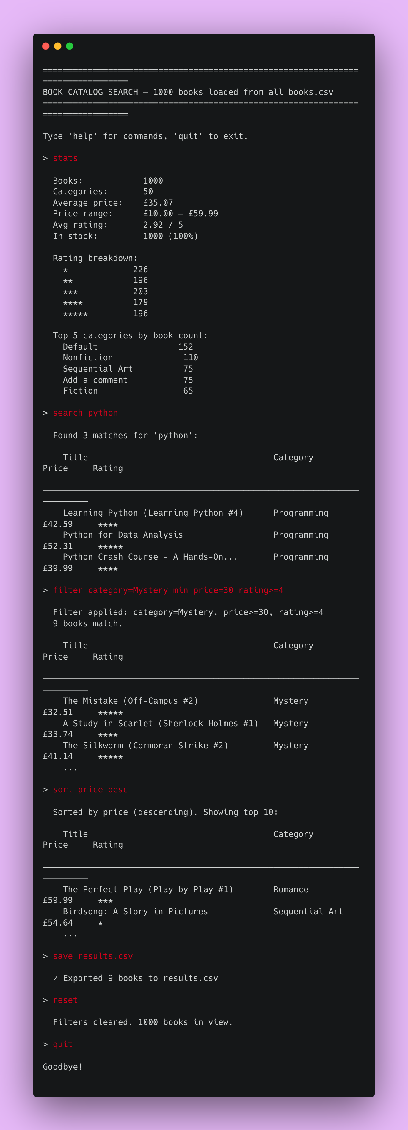
You drop a search command and your dataset answers. Combine filters and it slices in real time. That’s a tool.

Setup Instructions

Install pandas:

pip install pandas

(You also need all_books.csv — the output of Day 2. If you haven’t run that yet, run it first, or use the sample file provided below)

Run the program:

python search_books.py

The tool drops you into an interactive prompt. Type help to see the commands; type quit to exit.

Understanding the REPL Loop

A REPL — Read, Evaluate, Print, Loop — is just a while loop around input() and a dispatch on what the user typed. It’s the simplest way to build an interactive tool, and it suits this kind of dataset exploration perfectly:

def run_repl(df):
    current = df  # the current "view" - starts as the whole dataset

    while True:
        line = input("> ").strip()
        if not line:
            continue
        if line == "quit":
            break

        # parse the command and dispatch
        current = handle_command(line, df, current)

Three habits worth noticing:

• An empty line just continues — common enough to handle explicitly.

• The user typed string is .strip()ped — trailing whitespace from a paste shouldn’t break commands.

• current holds the filtered view, separate from df (the full catalog) — so reset always has the full data to return to.

Understanding Command Parsing

Each command starts with a word (search, filter, sort, stats...) followed by arguments. The simplest parse: split on whitespace, take the first token as the command name:

def handle_command(line, df, current):
    parts = line.split()
    cmd = parts[0].lower()
    args = parts[1:]

    if cmd == "search":
        return command_search(current, " ".join(args))
    if cmd == "filter":
        return command_filter(df, args)
    if cmd == "stats":
        command_stats(current)
        return current
    # ...

Each command gets its own function. command_search and command_filter return the new view (so the REPL can update current); command_stats just prints and returns the view unchanged. This keeps the dispatch readable — each command does one thing in one place.

Understanding pandas String Search

The search command should match across titles and descriptions, case-insensitively. pandas’ .str.contains() does the heavy lifting:

def command_search(df, query):
    if not query:
        print("  Usage: search <keyword>")
        return df

    title_match = df["title"].str.contains(query, case=False, na=False)
    desc_match = df["description"].str.contains(query, case=False, na=False)

    matches = df[title_match | desc_match]
    show_results(matches, f"Found {len(matches)} matches for '{query}'")
    return matches

A few important details:

• case=False — case-insensitive matching. "python" finds "Python".

• na=False — treats missing values as “no match” instead of NaN. Without it, you get errors when the column has any blanks.

• | — boolean OR between the two masks. A book matches if either the title or the description contains the keyword.

The result is a new DataFrame — a filtered view of the catalog — that becomes the new current. The next command operates on those matches.

Understanding Boolean Masks

Filtering in pandas is built on boolean masks: a column of True/False the same length as the DataFrame, used to keep only the True rows.

# Books over £30
mask = df["price"] >= 30
expensive = df[mask]

# Books over £30 AND rated 4+
mask = (df["price"] >= 30) & (df["rating"] >= 4)
expensive_and_good = df[mask]

Two non-obvious rules every pandas user hits:

• Use & and |, not and and or. The Python keywords don’t work on column-level booleans.

• Wrap each condition in parentheses. & has higher precedence than >=, so without parens the order is wrong and you get errors.

(condition) & (condition) & (condition) is how every multi-filter query in pandas looks. Get used to it.

Understanding the Filter Command

The filter command takes key-value pairs like category=Fiction min_price=20 rating>=4. We parse each piece, build a list of conditions, then combine them:

def command_filter(df, args):
    mask = pd.Series(True, index=df.index)   # start: keep everything
    applied = []

    for arg in args:
        if arg.startswith("category="):
            value = arg.split("=", 1)[1].lower()
            mask &= df["category"].str.lower().str.contains(value, na=False)
            applied.append(f"category={value}")

        elif arg.startswith("min_price="):
            value = float(arg.split("=", 1)[1])
            mask &= df["price"] >= value
            applied.append(f"price>={value}")

        elif arg.startswith("max_price="):
            value = float(arg.split("=", 1)[1])
            mask &= df["price"] <= value
            applied.append(f"price<={value}")

        elif arg.startswith("rating>="):
            value = int(arg.split("=", 1)[1])
            mask &= df["rating"] >= value
            applied.append(f"rating>={value}")

    result = df[mask]
    print(f"  Filter applied: {', '.join(applied)}")
    show_results(result, f"{len(result)} books match.")
    return result

Two patterns worth taking away:

• Build masks incrementally with &= — starting from True everywhere, each condition narrows the result. Whether the user passes one filter or four, the same loop handles it.

• Always re-filter from the full catalog, not the current view. That way filter category=Fiction replaces the previous filter rather than narrowing within it — usually what you actually want.

Understanding the Sort Command

sort price desc reorders the current view. The parse picks up the column and direction:

def command_sort(df, args):
    if not args:
        print("  Usage: sort <field> [asc|desc]")
        return df

    field = args[0]
    ascending = not (len(args) > 1 and args[1].lower() == "desc")

    if field not in df.columns:
        print(f"  Unknown field: {field}")
        return df

    sorted_df = df.sort_values(field, ascending=ascending).head(10)
    direction = "ascending" if ascending else "descending"
    print(f"  Sorted by {field} ({direction}). Showing top 10:")
    show_results(sorted_df, "")
    return df  # return original; don't permanently sort the view

A subtlety: sort should display the sorted top-10 but not change the filter state. So we show the sorted view, but return the unsorted current view. The user expects “show me the top by price” to be a view, not a state change — the next filter shouldn’t be operating on a sliced sorted list.

Understanding Formatting Aligned Output

A search result is just a DataFrame — but print(df) looks ugly. We format each row manually so titles align, prices line up by the decimal, and ratings use stars:

def show_results(df, header_message):
    if header_message:
        print(f"\n  {header_message}")
    if df.empty:
        print("  (no results)")
        return

    print()
    print(f"    {'Title':<40} {'Category':<18} {'Price':>8} {'Rating':>10}")
    print("    " + "─" * 80)

    for _, row in df.head(20).iterrows():
        title = row["title"]
        if len(title) > 40:
            title = title[:37] + "..."
        stars = "★" * int(row["rating"])
        print(f"    {title:<40} {row['category']:<18} "
              f"£{row['price']:>6.2f}   {stars:>8}")

.head(20) caps the output — nobody scrolls through 1,000 rows in a terminal. The column widths (:<40, :<18, :>8) and right-aligned price with two decimals (>6.2f) make the table read like a real product, not raw data.

Understanding the Stats Command

stats runs on the current view, so the same command answers both “stats for the full catalog” and “stats for what I just filtered.” It’s all pandas aggregation:

def command_stats(df):
    if df.empty:
        print("  No books in current view.")
        return

    print(f"\n  Books:            {len(df)}")
    print(f"  Categories:       {df['category'].nunique()}")
    print(f"  Average price:    £{df['price'].mean():.2f}")
    print(f"  Price range:      £{df['price'].min():.2f} – £{df['price'].max():.2f}")
    print(f"  Avg rating:       {df['rating'].mean():.2f} / 5")
    in_stock = (df["stock_count"] > 0).sum()
    print(f"  In stock:         {in_stock} ({in_stock / len(df) * 100:.0f}%)")

    print("\n  Rating breakdown:")
    for rating in range(1, 6):
        count = (df["rating"] == rating).sum()
        stars = "★" * rating
        print(f"    {stars:<13} {count:>3}")

    print("\n  Top 5 categories by book count:")
    top = df["category"].value_counts().head(5)
    for cat, count in top.items():
        print(f"    {cat:<22} {count:>3}")

The reusable trick: df['category'].value_counts() — counts how often each value appears, sorted descending, in one line. It’s the fastest way to build a “top categories” or “top X” list from any column.

Understanding the Export Command

save results.csv writes the current view to a file. One line:

def command_save(df, args):
    if not args:
        print("  Usage: save <filename>")
        return df
    path = args[0]
    df.to_csv(path, index=False)
    print(f"  ✓ Exported {len(df)} books to {path}")
    return df

This is the closing of the loop: scrape → enrich → query → export the answer. The user can take their filtered subset into pandas, Excel, or another tool. The tool becomes a gateway, not just an endpoint.

Understanding Graceful Error Handling

Users mistype things. A REPL that crashes on a typo is unusable, so each command wraps its risky parts in try/except:

try:
    value = float(arg.split("=", 1)[1])
except ValueError:
    print(f"  Could not parse: {arg}")
    continue

The unknown-command fallback is just as important — help is a single press away, and bad input is just a printed message:

print(f"  Unknown command: {cmd}. Type 'help' for the list.")

Quiet, clear, forgiving. A tool you’d actually use.

Understanding Why This Is the Right Finale

Look at the three days together:

• Day 1 taught you to extract from one page.

• Day 2 taught you to scale across many pages with pagination and detail-page enrichment.

• Day 3 taught you to use the result — turning raw scraped data into answers.

The arc matters: scraping by itself isn’t valuable, it’s the dataset and what you do with it that matters. Every real scraping project ends with a query interface, a dashboard, an analysis — something that turns rows into decisions. Today’s REPL is the smallest, simplest version of that, and it makes the whole week click into place.

What You’ve Accomplished This Week

🎉 Congratulations! You’ve built a complete web scraping pipeline:

• Day 1: Extract structured data from a single web page

• Day 2: Scale across pagination + detail pages, with polite delays

• Day 3: Turn the scraped catalog into an interactive search tool

You now have:

✅ Scraping fundamentals — requests, BeautifulSoup, CSS class selection, attributes ✅ Pagination and multi-level scraping — listing pages + detail pages, combined cleanly ✅ Polite scraping habits — User-Agent, timeouts, delays, error handling ✅ Querying skills with pandas — boolean masks, string search, sorting, aggregation ✅ A real tool — your scraped data, queryable in real time

Next steps:

• Add a charts module: matplotlib distribution plots for price and rating

• Persist the dataset to SQLite for fast queries on larger catalogs

• Build a Streamlit version of the query interface

• Add a watcher: nightly rescrape, diff against the previous CSV

• Handle login-required sites with requests.Session

You’ve built the foundation for a real scraping-and-analysis pipeline. 🚀

View Code Evolution

Compare today’s query tool with Day 1’s single-page scraper and Day 2’s full-catalog scraper — and see how a clean three-step pipeline (extract → scale → query) is the shape of every real scraping project.