World Cup 2026 Match Predictor: Day 2- Poisson Goal Model

Learn how to use the Poisson goal model to predict each team’s goals drawn from a probability distribution, with rates estimated from recent form of each team.

Projects in this week’s series:

This week, we build a World Cup 2026 Match Predictor — a Streamlit web app that predicts upcoming matches using real football-analytics techniques. Each day the same interface stays, but the model behind it gets smarter.

• Day 1: Elo-based Predictor

• Day 2: Poisson Goal Model (Today)

• Day 3: Ensemble + Interactive Analysis

View All Projects This Week

Today’s Project

Yesterday’s Elo model was good at one thing: telling us who is likely to win. But football fans care about more than that — they want to know how it’ll go. Will it be a rout or a close game? What’s the most likely scoreline? What’s the chance of a draw?

Today we add all of that. The Poisson goal model treats each team’s goals as random events drawn from a probability distribution, with rates estimated from recent form. From that we get:

• Expected goals (λ) for each team — the rate parameter

• A full grid of scoreline probabilities

• W / D / L split — draws now have their own line

• The most likely exact scoreline

Same Streamlit UI, better answers.

The Big Idea Behind Poisson

Football goals aren’t uniformly distributed. Teams don’t score exactly 1.5 goals per match — they score 0, 1, 2, sometimes 5, occasionally none. But the average rate over many matches is measurable, and the distribution of individual match totals around that average follows a very specific pattern.

That pattern is the Poisson distribution — the standard model for “count of independent events over a fixed period.” Radioactive decay, phone calls per hour to a call center, and football goals per team per match all follow the same shape.

The Poisson distribution says: if a team’s average scoring rate is λ (lambda), the probability they score exactly k goals in one match is:

$$P(k) = \frac{e^{-\lambda} \lambda^k}{k!}$$

For a team averaging 1.5 goals per match:

• Probability of 0 goals: 22%

• Probability of 1 goal: 33%

• Probability of 2 goals: 25%

• Probability of 3 goals: 13%

• Probability of 4 goals: 5%

Sums to essentially 100% (the tail is tiny). That’s it — one number (λ) fully describes a team’s scoring profile.

Project Task

Extend yesterday’s app so it:

• Estimates each team’s attack strength (goals scored vs league average) and defense strength (goals conceded vs league average) from recent matches

• Computes expected goals (λ) for each team in a matchup

• Builds a scoreline probability matrix using two independent Poisson distributions

• Sums the matrix into W / D / L probabilities

• Finds the most likely exact scoreline

• Displays all of the above in the same card-based Streamlit UI as Day 1

• Shows a sidebar of top-20 WC 2026 teams by attack strength

Expected Output

Running the app:

streamlit run predictor_poisson.py

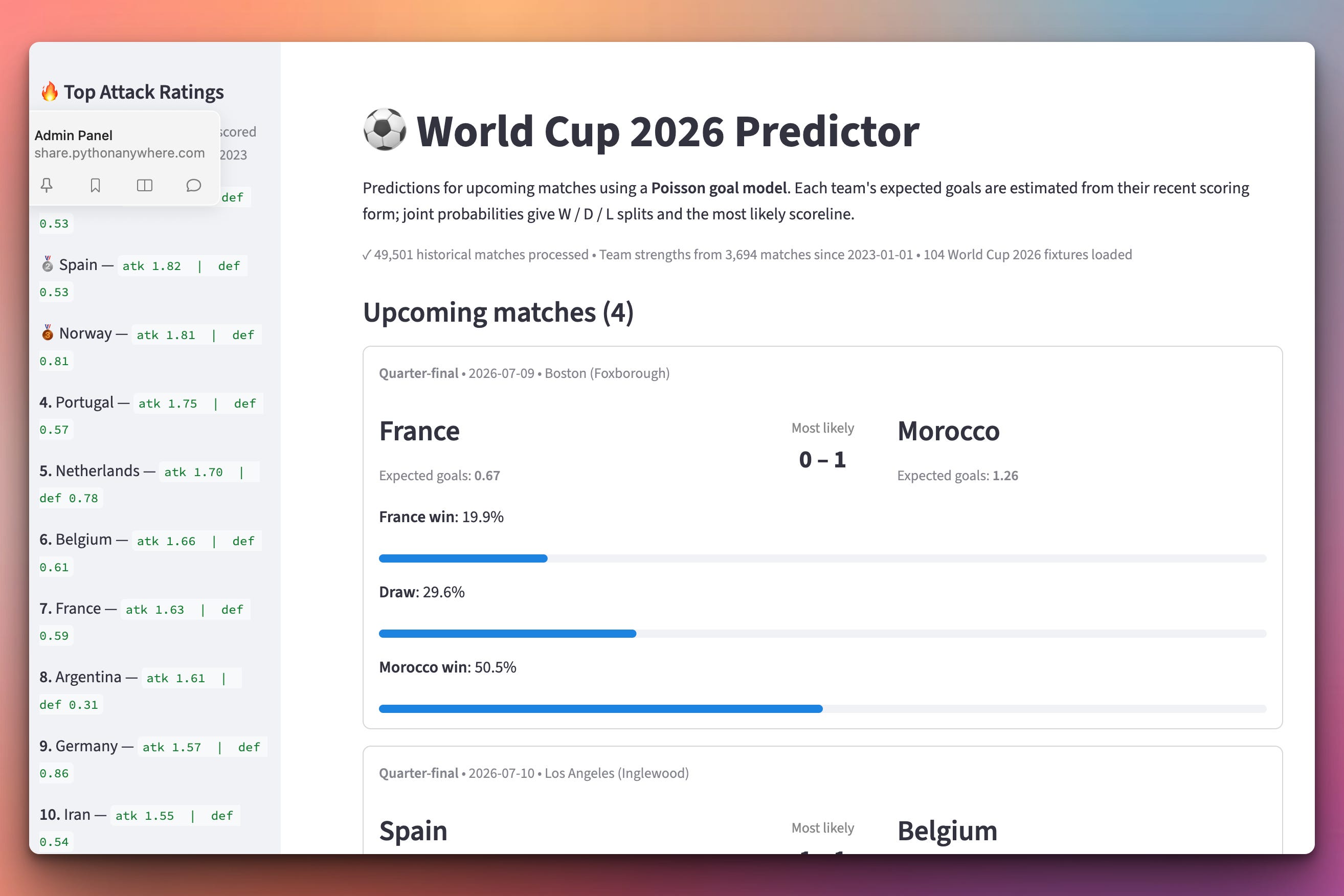
Why is Morocco predicted to win here?

The screenshot above shows France vs Morocco in the Quarter-final. The app predicts Morocco to win at 50.5%, with a most likely scoreline of 0–1. If you’re a football fan you’re probably surprised — France is clearly the “bigger” team, right? So what’s going on?

The Poisson model looks at each team’s recent scoring form since 2023, not their historical prestige. And when you look at the actual numbers:

• France has an attack strength of 1.63 (63% above the international average of 1.4 goals/match) and a defense strength of 0.59.

• Morocco has an attack strength of 1.53 — very close to France — but a defense strength of 0.29. They’ve conceded just 23 goals in 56 matches since 2023.

That defense number is the whole story. Morocco has been exceptionally stingy defensively — including drawing Brazil 1-1 and Netherlands 1-1 in the group stage, and beating Canada 3-0 in the Round of 16. When we multiply France’s attack × Morocco’s tiny defense number, France’s expected goals collapses to 0.67. Meanwhile Morocco’s attack × France’s more permissive defense gives Morocco 1.26 expected goals.

The prediction reflects a specific truth: over the last 3 years, Morocco’s defensive record is elite, and France’s attack has been less prolific than reputation suggests. Whether that translates to a real Morocco win is up to Wednesday — the model captures a real signal but ignores things like tournament pressure and historical class.

This tension between “recent form” and “long-term class” is exactly why we’re building an ensemble on Day 3. Yesterday’s Elo model, which uses every match since 1872, still favors France at 68%. When the two models disagree like this, the truth usually lies in the middle.

Setup Instructions

Nothing new to install — same dependencies as Day 1.

pip install streamlit requests
streamlit run predictor_poisson.py

Understanding Team Attack and Defense Strength

Before the Poisson math can happen, we need to estimate each team’s scoring rate. But teams don’t play in a vacuum — a 3-0 win is impressive against a strong opponent, meaningless against a minnow. The trick is to normalize by opponent strength using multiplicative factors:

def compute_team_strength(matches):
    recent = [m for m in matches if m["date"] >= FORM_WINDOW_START]

    scored = defaultdict(list)
    conceded = defaultdict(list)

    for m in recent:
        hg, ag = int(m["home_score"]), int(m["away_score"])
        home, away = m["home_team"], m["away_team"]
        scored[home].append(hg)
        scored[away].append(ag)
        conceded[home].append(ag)
        conceded[away].append(hg)

    strength = {}
    for team in scored:
        avg_scored = sum(scored[team]) / len(scored[team])
        avg_conceded = sum(conceded[team]) / len(conceded[team])
        strength[team] = {
            "attack":  avg_scored / LEAGUE_AVG_GOALS,
            "defense": avg_conceded / LEAGUE_AVG_GOALS,
        }

    return strength

The output is two multipliers per team:

• attack = 1.0 — you score at league average.

• attack = 1.5 — you score 50% more than league average.

• defense = 0.7 — you concede 30% less than league average (defense good; the lower the number, the tighter the defense).

Real numbers from live data: Japan attack 2.02, defense 0.53 (dominant scoring, stingy defense). Spain attack 1.82, defense 0.53 (elite). These are relative to the international average of 1.4 goals per team per match.

Understanding the Sample Size Guard

There’s a classic gotcha here that will bite you the first time you build a ranking like this: teams with very few matches will dominate the top of the list. If you rank the whole world of national teams by attack strength, the top 20 gets flooded with tiny CONIFA teams — Isle of Man, Tamil Eelam, Jersey, Sápmi — all of whom play maybe 6-10 matches every few years against similarly small teams and end up with wildly inflated attack numbers.

The naive fix is a minimum-matches filter (s["matches"] >= 30). But we can do something cleaner and more relevant to our specific app: only show teams that are actually at the World Cup 2026.

def wc_teams(fixtures):
    """The set of real (non-placeholder) team names in the WC 2026 fixtures."""
    teams = set()
    for m in fixtures["matches"]:
        for name in (m["team1"], m["team2"]):
            if not is_placeholder(name):
                teams.add(name)
    return teams

# In the sidebar:
qualifying = {t: s for t, s in strength.items() if t in wc_team_set}
top = sorted(qualifying.items(), key=lambda x: -x[1]["attack"])[:20]

Two lines. But this is a much better solution than a raw sample-size filter for two reasons:

• It’s semantically correct. This is a World Cup app; only WC teams belong in the sidebar. Isle of Man’s attack strength is irrelevant to anyone using this tool.

• It solves the noise problem automatically. Every WC team has played ~40+ international matches since 2023 (they had to qualify, they play friendlies, they’re in continental competitions). The 48 WC teams are automatically the sample-size-clean subset.

The lesson: the right filter is often a domain filter, not a technical one. Instead of “teams with 30+ matches” (arbitrary threshold), we filter by “teams that matter for this specific view” (natural, defensible boundary). Any time you’re about to reach for a magic number to filter noise, ask first if there’s a domain fact that does the same job cleanly.

We still compute strengths for every team (Morocco’s defense number needs their whole history, not just their WC record) — we’re just choosing not to display the ones that aren’t relevant.

Understanding the Recent-Form Window

We only look at matches since a cutoff date:

FORM_WINDOW_START = "2023-01-01"

Why? Because a team’s 2010 attack strength doesn’t tell us much about their 2026 form. Coaches change, players retire, tactics evolve. Three years is the sweet spot for international football — enough matches to be meaningful (~40-50 per top team), recent enough to reflect current reality.

Compare this with Day 1’s Elo, which used every match ever. That’s the right choice for Elo — the rating evolves gradually with each result, so the current rating already captures recent form. For Poisson, we need a fresh per-team average, so a rolling window works better.

Different models want different data. That’s the meta-lesson of doing two models.

Understanding Expected Goals (Lambda)

Given both teams’ attack and defense multipliers, the expected goals for a matchup is a three-way product:

def expected_goals(team1, team2, strength):
    s1 = strength[team1]
    s2 = strength[team2]
    lambda1 = s1["attack"] * s2["defense"] * LEAGUE_AVG_GOALS
    lambda2 = s2["attack"] * s1["defense"] * LEAGUE_AVG_GOALS
    return lambda1, lambda2

The formula in plain English:

Team1’s expected goals = (how well they score) × (how easy team2 is to score against) × (the average goals in a match).

For France vs Morocco: France’s expected goals = France’s attack (1.63) × Morocco’s defense (0.29) × 1.4 = 0.67 (very low, because Morocco is so hard to score against). Morocco’s expected goals = Morocco’s attack (1.53) × France’s defense (0.59) × 1.4 = 1.26. Morocco is the Poisson favorite despite being lower-Elo.

This is why the models disagree. Elo bakes in the whole history; Poisson listens to what’s happened recently. Both perspectives are legitimate.

Understanding the Poisson PMF

The probability mass function for a Poisson distribution:

from math import exp, factorial

def poisson_pmf(k, lam):
    """Probability of exactly k events when the rate is lam."""
    return exp(-lam) * (lam ** k) / factorial(k)

That’s the whole math. Three built-in Python operations: exp, **, factorial. No NumPy, no SciPy, no dependencies beyond stdlib.

For λ = 1.5:

• poisson_pmf(0, 1.5) = 0.223 → 22% chance of 0 goals

• poisson_pmf(1, 1.5) = 0.335 → 33% chance of 1 goal

• poisson_pmf(2, 1.5) = 0.251 → 25% chance of 2 goals

• poisson_pmf(3, 1.5) = 0.126 → 13% chance of 3 goals

Sum: 93% by k=3, essentially 100% by k=5. Football scores are dominated by low numbers, and Poisson captures that shape naturally.

Understanding the Scoreline Matrix

To predict a match outcome, we build a joint probability grid — every possible scoreline gets a probability:

def score_matrix(lambda1, lambda2, max_goals=8):
    matrix = {}
    for g1 in range(max_goals + 1):
        p1 = poisson_pmf(g1, lambda1)
        for g2 in range(max_goals + 1):
            p2 = poisson_pmf(g2, lambda2)
            matrix[(g1, g2)] = p1 * p2
    return matrix

The critical assumption: team1’s goals and team2’s goals are independent. So P(1-0) = P(team1 scores 1) × P(team2 scores 0).

For most matches this assumption holds well enough. Real matches have some correlation (a team that’s winning big might ease off; a team that’s losing might risk more) but the independence assumption is a reasonable first-order model. Dixon and Coles’ famous 1997 improvement adjusted for exactly this correlation in 0-0 and 1-1 outcomes; you can bolt it on later.

max_goals=8 is our practical upper bound. The probability of any score beyond 8-8 is astronomically tiny; ignoring it costs us less than 0.01% of the total probability.

Understanding the Most-Likely Scoreline

Finding the single most-probable scoreline is a one-liner using max with a key:

def most_likely_score(matrix):
    return max(matrix, key=matrix.get)

matrix.get is the accessor that returns the probability for a given key; max(..., key=fn) returns the key whose function-value is largest. Python at its most elegant.

For Argentina vs Egypt (Argentina expected goals 1.30, Egypt 0.50), the top 5 scorelines are:

Score Probability 1-0 21.4% 0-0 16.5% 2-0 13.9% 1-1 10.8% 0-1 8.3%

The most likely single score is 1-0, but even the most likely score only happens 21% of the time — football is inherently high-variance. That’s why we care about probability distributions and not just point predictions.

Understanding the Model’s Limitations

Every model has weaknesses. Poisson’s are worth naming — and are exactly why the France vs Morocco prediction feels off:

1. Independence assumption: teams’ goals aren’t perfectly independent. Real matches have correlation — winning teams ease off, losing teams take risks. Dixon-Coles (1997) fixes this by adjusting the corners of the matrix.

2. Opponent quality isn’t weighted: we compute attack as raw goals scored / league average, without weighting by who was defended against. So a team that mostly plays weaker opponents will look artificially strong. Morocco’s 5-0 friendly rout of Burundi counts the same as their 1-1 vs Brazil.

3. Match importance isn’t weighted: friendlies count the same as World Cup matches. A team that runs up scores in exhibitions inflates its attack rating.

4. No context: injuries, tournament pressure, weather — none of it’s in the model.

Every one of these is fixable with more work. But even this vanilla Poisson model produces ~62% match-outcome accuracy in the football-analytics literature. Good baseline. The interesting question is what happens when we combine it with Elo — which has different blind spots.

Understanding Comparing the Models

Here’s what makes tomorrow interesting. Look at these live matchups from right now:

Match Elo says Poisson says France vs Morocco France 68% Morocco 51% Norway vs England England 64% England 51% Spain vs Belgium Spain 72% Spain 45% / Draw 25% / Belgium 30% Argentina vs Switzerland Argentina 78% Argentina 63%

Elo is confident. Poisson is more uncertain. And sometimes they disagree entirely on the favorite.

Which one is right? Both, and neither. Elo sees the long game (decades of results); Poisson listens to recent form (this year’s goals). When they agree, we can be confident. When they disagree, we should probably say so.

That’s the whole motivation for tomorrow’s ensemble — combining the two models into one prediction, and showing the user when the models are aligned vs when they’re arguing.

Coming Tomorrow

Tomorrow the two models meet. We build an ensemble — a weighted average of Elo and Poisson probabilities — that outperforms either alone. And we add interactivity: click any match card and expand it to see both model’s answers side-by-side, the recent form of each team (W-W-D-L-W last 5), and a confidence indicator that tells you when the models agree vs when they’re arguing. The finale is where it all clicks.

View Code Evolution

Compare today’s Poisson predictor with Day 1’s Elo predictor and see how a fundamentally different mathematical model plugs into the same UI shell — because we designed the UI to be model-agnostic from day one.